Dynamic Topic Models Tutorial
What is this tutorial about?
This tutorial will exaplin what Dynamic Topic Models are, and how to use them using the LdaSeqModel class of gensim. I will start with some theory and already documented examples, before moving on to an example run of Dynamic Topic Model on a sample dataset. I will also do an comparison between the python code and the already present gensim wrapper, and illustrate how to easily visualise them and do topic coherence with DTM. Any suggestions to improve documentation or code through PRs/Issues is always appreciated!
Why Dynamic Topic Models?
Imagine you have a gigantic corpus which spans over a couple of years. You want to find semantically similar documents; one from the very beginning of your time-line, and one in the very end. How would you? This is where Dynamic Topic Models comes in. By having a time-based element to topics, context is preserved while key-words may change.
David Blei does a good job explaining the theory behind this in this Google talk. If you prefer to directly read the paper on DTM by Blei and Lafferty, that should get you upto speed too.
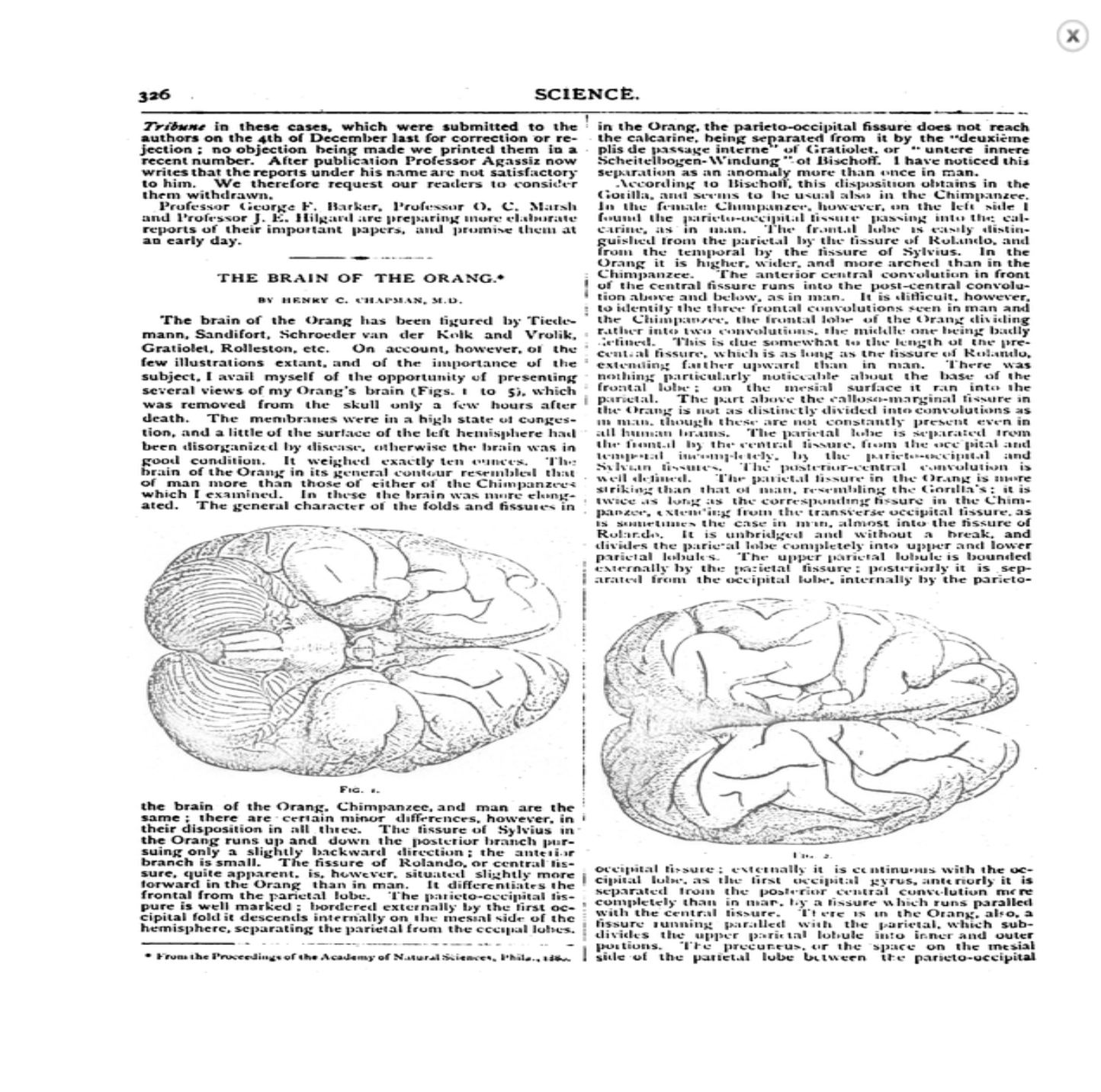
In his talk, Blei gives a very interesting example of the motivation to use DTM. After running DTM on a dataset of the Science Journal from 1880 onwards, he picks up this paper - The Brain of the Orang (1880). It's topics are concentrated on a topic which must be to do with Monkeys, and with Neuroscience or brains.
He goes ahead to pick up another paper with likely very less common words, but in the same context - analysing monkey brains. In fact, this one is called - "Representation of the visual field on the medial wall of occipital-parietal cortex in the owl monkey". Quite the title, eh? Like mentioned before, you wouldn't imagine too many common words in these two papers, about a 100 years apart.
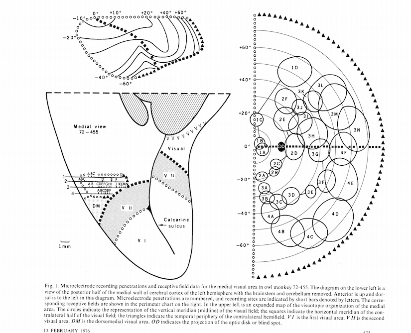
But a Hellinger Distance based Document-Topic distribution gives a very high similarity value! The same topics evolved smoothly over time and the context remains. A document similarity match using other traditional techniques might not work very well on this! Blei defines this technique as - "Time corrected Document Similarity".
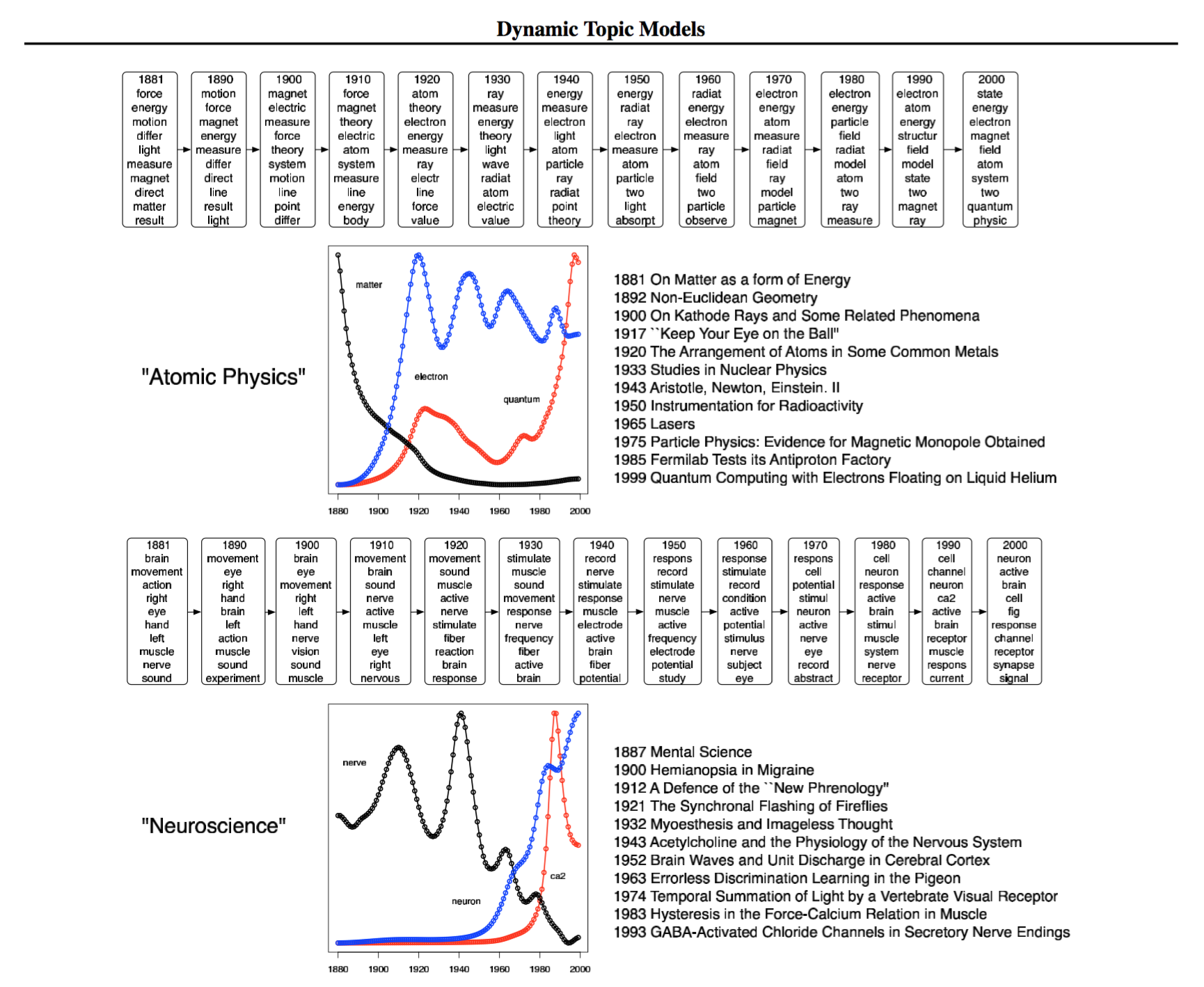
Another obviously useful analysis is to see how words in a topic change over time. The same broad classified topic starts looking more 'mature' as time goes on. This image illustrates an example from the same paper linked to above.
So, briefly put :
Dynamic Topic Models are used to model the evolution of topics in a corpus, over time. The Dynamic Topic Model is part of a class of probabilistic topic models, like the LDA.
While most traditional topic mining algorithms do not expect time-tagged data or take into account any prior ordering, Dynamic Topic Models (DTM) leverages the knowledge of different documents belonging to a different time-slice in an attempt to map how the words in a topic change over time.
This blog post is also useful in breaking down the ideas and theory behind DTM.
Motivation to code this!
But - why even undertake this, especially when Gensim itself have a wrapper? The main motivation was the lack of documentation in the original code - and the fact that doing an only python version makes it easier to use gensim building blocks. For example, for setting up the Sufficient Statistics to initialize the DTM, you can just pass a pre-trained gensim LDA model!
There is some clarity on how they built their code now - Variational Inference using Kalman Filters, as described in section 3 of the paper. The mathematical basis for the code is well described in the appendix of the paper. If the documentation is lacking or not clear, comments via Issues or PRs via the gensim repo would be useful in improving the quality.
This project was part of the Google Summer of Code 2016 program: I have been regularly blogging about my progress with implementing this, which you can find here.
Using LdaSeqModel for DTM
Gensim already has a wrapper for original C++ DTM code, but the LdaSeqModel class is an effort to have a pure python implementation of the same.
Using it is very similar to using any other gensim topic-modelling algorithm, with all you need to start is an iterable gensim corpus, id2word and a list with the number of documents in each of your time-slices.
# setting up our imports

from gensim.models import ldaseqmodel
from gensim.corpora import Dictionary, bleicorpus
import numpy
from gensim.matutils import hellinger
We will be loading the corpus and dictionary from disk. Here our corpus in the Blei corpus format, but it can be any iterable corpus. The data set here consists of news reports over 3 months (March, April, May) downloaded from here and cleaned.
The files can also be found after processing in the datasets folder, but it would be a good exercise to download the files in the link and have a shot at cleaning and processing yourself. :)
Note: the dataset is not cleaned and requires pre-processing. This means that some care must be taken to group the relevant docs together (the months are mentioned as per the folder name), after which it needs to be broken into tokens, and stop words must be removed. This is a link to some basic pre-processing for gensim - link.
What is a time-slice?
A very important input for DTM to work is the time_slice input. It should be a list which contains the number of documents in each time-slice. In our case, the first month had 438 articles, the second 430 and the last month had 456 articles. This means we'd need an input which looks like this: time_slice = [438, 430, 456].
Technically, a time-slice can be a month, year, or any way you wish to split up the number of documents in your corpus, time-based.
Once you have your corpus, id2word and time_slice ready, we're good to go!
# loading our corpus and dictionary
try:
    dictionary = Dictionary.load('datasets/news_dictionary')
except FileNotFoundError as e:
    raise ValueError("SKIP: Please download the Corpus/news_dictionary dataset.")
corpus = bleicorpus.BleiCorpus('datasets/news_corpus')
# it's very important that your corpus is saved in order of your time-slices!

time_slice = [438, 430, 456]
For DTM to work it first needs the Sufficient Statistics from a trained LDA model on the same dataset. By default LdaSeqModel trains it's own model and passes those values on, but can also accept a pre-trained gensim LDA model, or a numpy matrix which contains the Suff Stats.
We will be training our model in default mode, so gensim LDA will be first trained on the dataset.
NOTE: You have to set logging as true to see your progress!
ldaseq = ldaseqmodel.LdaSeqModel(corpus=corpus, id2word=dictionary, time_slice=time_slice, num_topics=5)
Now that our model is trained, let's see what our results look like.
Results
Much like LDA, the points of interest would be in what the topics are and how the documents are made up of these topics. In DTM we have the added interest of seeing how these topics evolve over time.
Let's go through some of the functions to print Topics and analyse documents.
Printing Topics
To print all topics from a particular time-period, simply use print_topics.
The input parameter to print_topics is a time-slice option. By passing 0 we are seeing the topics in the 1st time-slice.
The result would be a list of lists, where each individual list contains a tuple of the most probable words in the topic. i.e (word, word_probability)
ldaseq.print_topics(time=0)
We can see 5 different fairly well defined topics:
- Economy
- Entertainment
- Football
- Technology and Entertainment
- Government
Looking for Topic Evolution
To fix a topic and see it evolve, use print_topic_times.
The input parameter is the topic_id
In this case, we are looking at the evolution of the technology topic.
If you look at the lower frequencies; the word "may" is creeping itself into prominence. This makes sense, as the 3rd time-slice are news reports about the economy in the month of may. This isn't present at all in the first time-slice because it's still March!
ldaseq.print_topic_times(topic=0) # evolution of 1st topic
Document - Topic Proportions
the function doc_topics checks the topic proportions on documents already trained on. It accepts the document number in the corpus as an input.
Let's pick up document number 558 arbitrarily and have a look.
# to check Document - Topic proportions, use `doc-topics`
words = [dictionary[word_id] for word_id, count in corpus[558]]
print (words)
It's pretty clear that it's a news article about football. What topics will it likely be comprised of?
doc = ldaseq.doc_topics(558) # check the 558th document in the corpuses topic distribution
print (doc)
Let's look at our topics as desribed by us, again:
- Economy
- Entertainment
- Football
- Technology and Entertainment
- Government
Our topic distribution for the above document is largely in topics 3 and 4. Considering it is a document about a news article on a football match, the distribution makes perfect sense!
If we wish to analyse a document not in our training set, we can use simply pass the doc to the model similar to the __getitem__ funciton for LdaModel.
Let's let our document be a hypothetical news article about the effects of Ryan Giggs buying mobiles affecting the British economy.
doc_football_1 = ['economy', 'bank', 'mobile', 'phone', 'markets', 'buy', 'football', 'united', 'giggs']
doc_football_1 = dictionary.doc2bow(doc_football_1)
doc_football_1 = ldaseq[doc_football_1]
print (doc_football_1)
Pretty neat! Topic 1 is about the Economy, and this document also has traces of football and technology, so topics 1, 3, and 4 got correctly activated.
Distances between documents
One of the more handy uses of DTMs topic modelling is that we can compare documents across different time-frames and see how similar they are topic-wise. When words may not necessarily overlap over these time-periods, this is very useful.
The current dataset doesn't provide us the diversity for this to be an effective example; but we will nevertheless illustrate how to do the same.
doc_football_2 = ['arsenal', 'fourth', 'wenger', 'oil', 'middle', 'east', 'sanction', 'fluctuation']
doc_football_2 = dictionary.doc2bow(doc_football_2)
doc_football_2 = ldaseq[doc_football_2]
hellinger(doc_football_1, doc_football_2)
The topic distributions are quite related - matches well in football and economy.
Now let's try with documents that shouldn't be similar.
doc_governemt_1 = ['tony', 'government', 'house', 'party', 'vote', 'european', 'official', 'house']
doc_governemt_1 = dictionary.doc2bow(doc_governemt_1)
doc_governemt_1 = ldaseq[doc_governemt_1]

hellinger(doc_football_1, doc_governemt_1)
As expected, the value is very high, meaning the topic distributions are far apart.
For more information on how to use the gensim distance metrics, check out this notebook.
Performance
The code currently runs between 5 to 7 times slower than the original C++ DTM code. The bottleneck is in the scipy optimize.fmin_cg method for updating obs. Speeding this up would fix things up!
Since it uses iterable gensim corpuses, the memory stamp is also cleaner.
TODO: check memory, check BLAS, see how performance can be improved memory and speed wise.
The advantages of the python port are that unlike the C++ code we needn't treat it like a black-box; PRs to help make the code better are welcomed, as well as help to make the documentation clearer and improve performance. It is also in pure python and doesn't need any dependancy outside of what gensim already needs. The added functionality of being able to analyse new documents is also a plus!
Choosing your best Dynamic Topic Model.
Like we've been going on and on before, the advantage in having a python port is the transparency with which you can train your DTM. We'll go over two key ideas: changing variance, and changing suff stats.
Chain Variance
One of the key aspects of topic evolution is how fast/slow these topics evolve. And this is where the factor of variance comes in.
By setting the chain_variance input to the DTM model higher, we can tweak our topic evolution.
The default value is 0.005. (this is the value suggested by Blei in his tech talk and is the default value in the C++ code)
Let us see a small example illustrating the same. Let's first see the evolution of values for the first time-slice.
ldaseq.print_topic_times(1)
Now let us do the same, but after increasing the chain_variance value.
ldaseq_chain = ldaseqmodel.LdaSeqModel(corpus=corpus, id2word=dictionary, time_slice=time_slice, num_topics=5, chain_variance=0.05)
It's noticable that the values are moving more freely after increasing the chain_variance. Film went from highest probability to 5th to 8th!
ldaseq_chain.print_topic_times(2)
LDA Model and DTM
For the first slice of DTM to get setup, we need to provide it sufficient stats from an LDA model. As discussed before, this is done by fitting gensim LDA on the dataset first.
We also, however, have the option of passing our own model or suff stats values. Our final DTM results are heavily influenced by what we pass over here. We already know what a "Good" or "Bad" LDA model is (if not, read about it here).
It's quite obvious, then, that by passing a "bad" LDA model we will get not so satisfactory results; and by passing a better fitted or better trained LDA we will get better results. The same logic goes if we wish to directly pass the suff_stats numpy matrix.
Visualising Dynamic Topic Models.
Let us use pyLDAvis to visualise both the DTM wrapper and DTM python port.
With the new DTMvis methods it is now very straightforward to visualise DTM for a particular time-slice.
from gensim.models.wrappers.dtmmodel import DtmModel
from gensim.corpora import Dictionary, bleicorpus
import pyLDAvis

# dtm_path = "/Users/bhargavvader/Downloads/dtm_release/dtm/main"
# dtm_model = DtmModel(dtm_path, corpus, time_slice, num_topics=5, id2word=dictionary, initialize_lda=True)
# dtm_model.save('dtm_news')

# if we've saved before simply load the model
dtm_model = DtmModel.load('dtm_news')
If you take some time to look at the topics, you will notice large semantic similarities with the wrapper and the python DTM. Functionally, the python DTM replicates the wrapper quite well.
doc_topic, topic_term, doc_lengths, term_frequency, vocab = dtm_model.dtm_vis(time=0, corpus=corpus)
vis_wrapper = pyLDAvis.prepare(topic_term_dists=topic_term, doc_topic_dists=doc_topic, doc_lengths=doc_lengths, vocab=vocab, term_frequency=term_frequency)
pyLDAvis.display(vis_wrapper)
Now let us do the same for the python DTM.
In particular, look at topic 2 of the wrapper and topic 3 of the python port. Notice how they are both about football.
doc_topic, topic_term, doc_lengths, term_frequency, vocab = ldaseq.dtm_vis(time=0, corpus=corpus)
vis_dtm = pyLDAvis.prepare(topic_term_dists=topic_term, doc_topic_dists=doc_topic, doc_lengths=doc_lengths, vocab=vocab, term_frequency=term_frequency)
pyLDAvis.display(vis_dtm)
Visualising topics is a handy way to compare topic models.
Topic Coherence for DTM
Similar to visualising DTM time-slices, finding coherence values for both python DTM and the wrapper is very easy. We just have to specify the time-slice we want to find coherence for. The following examples will illustrate this.
from gensim.models.coherencemodel import CoherenceModel
import pickle

# we just have to specify the time-slice we want to find coherence for.
topics_wrapper = dtm_model.dtm_coherence(time=0)
topics_dtm = ldaseq.dtm_coherence(time=2)

# running u_mass coherence on our models
cm_wrapper = CoherenceModel(topics=topics_wrapper, corpus=corpus, dictionary=dictionary, coherence='u_mass')
cm_DTM = CoherenceModel(topics=topics_dtm, corpus=corpus, dictionary=dictionary, coherence='u_mass')

print ("U_mass topic coherence")
print ("Wrapper coherence is ", cm_wrapper.get_coherence())
print ("DTM Python coherence is", cm_DTM.get_coherence())

# to use 'c_v' we need texts, which we have saved to disk.
texts = pickle.load(open('Corpus/texts', 'rb'))
cm_wrapper = CoherenceModel(topics=topics_wrapper, texts=texts, dictionary=dictionary, coherence='c_v')
cm_DTM = CoherenceModel(topics=topics_dtm, texts=texts, dictionary=dictionary, coherence='c_v')

print ("C_v topic coherence")
print ("Wrapper coherence is ", cm_wrapper.get_coherence())
print ("DTM Python coherence is", cm_DTM.get_coherence())
Our values are a little behind the wrapper - but not by much.
Conclusion
So while there is already a python wrapper of DTM, a pure python implementation will be useful to better understand what goes on undcer the hood and tune our model. When it comes to performance, the C++ is undoubtedly faster, but we can continue to work on ours to make it as fast. As for evaluating the results, our topics are on par if not better than the wrapper!
On a more personal note, implementing Dynamic Topic Models with the Google Summer of Code 2016 program was a great learning experience. Gensim and RaRe Technologies have been a joy to work with, and Lev and Radim have been great mentors throughout, especially when things became slow or difficult. I look forward to continuing my contribution to gensim for a long time!